Apache Spark for data ingestion into Microsoft Fabric Lakehouse using Notebooks
Explore the power of Apache Spark and Python for seamless data ingestion into Microsoft Fabric Lakehouse. Dive into Fabric notebooks, a scalable and systematic solution that empowers you to ingest external data, configure authentication for external sources, and optimize your data loading process.

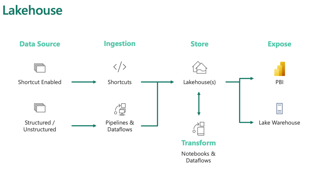
Apache Spark for Data Ingestion into Microsoft Fabric Lakehouse using Notebooks
Fabric Notebooks for Data Ingestion
- Automation and Efficiency: Fabric notebooks offer automated data ingestion, surpassing manual uploads and dataflows in handling large datasets.
- Location and Storage: These notebooks are stored within the workspace they are created in, which might differ from the lakehouse’s workspace.
- Functionality: They support multiple code and Markdown cells, ideal for testing and quick modifications. Individual cells can be run, frozen, or executed collectively.
Using PySpark in Fabric Notebooks
- Default Language: Fabric notebooks primarily use PySpark, leveraging the Spark engine for multi-threaded, distributed transactions, ensuring speed.
- Other Language Options: Although available, using Html, Spark (Scala), Spark SQL, and SparkR may not fully utilize the distributed system capabilities.
Connecting to Azure Blob Storage
# Azure Blob Storage access info
blob_account_name = "azureopendatastorage"
blob_container_name = "nyctlc"
blob_relative_path = "yellow"
blob_sas_token = "sv=2022-11-02&ss=bfqt&srt=c&sp=rwdlacupiytfx&se=2023-09-08T23:50:02Z&st=2023-09-08T15:50:02Z&spr=https&sig=abcdefg123456"

# Construct the path for connection
wasbs_path = f'wasbs://{blob_container_name}@{blob_account_name}.blob.core.windows.net/{blob_relative_path}?{blob_sas_token}'

# Read parquet data from Azure Blob Storage path
blob_df = spark.read.parquet(wasbs_path)

# Show the Azure Blob DataFrame
blob_df.show()
Connecting to External Data Sources
- Simplified Integration: Fabric notebooks provide easy integration with certain platforms, but require different methods for others.
- Example - Azure Blob Storage Connection:
- Define access information (account name, container name, relative path, SAS token).
- Create a connection path and use it to read data into a DataFrame.
- Display the data from Azure Blob Storage.
Connecting to Azure SQL Database with a Service Principal
# Placeholders for Azure SQL Database connection info
server_name = "your_server_name.database.windows.net"
port_number = 1433  # Default port number for SQL Server
database_name = "your_database_name"
table_name = "YourTableName" # Database table
client_id = "YOUR_CLIENT_ID"  # Service principal client ID
client_secret = "YOUR_CLIENT_SECRET"  # Service principal client secret
tenant_id = "YOUR_TENANT_ID"  # Azure Active Directory tenant ID

# Build the Azure SQL Database JDBC URL with Service Principal (Active Directory Integrated)
jdbc_url = f"jdbc:sqlserver://{server_name}:{port_number};database={database_name};encrypt=true;trustServerCertificate=false;hostNameInCertificate=*.database.windows.net;loginTimeout=30;Authentication=ActiveDirectoryIntegrated"

# Properties for the JDBC connection
properties = {
    "user": client_id,
    "password": client_secret,
    "driver": "com.microsoft.sqlserver.jdbc.SQLServerDriver",
    "tenantId": tenant_id
}

# Read entire table from Azure SQL Database using AAD Integrated authentication
sql_df = spark.read.jdbc(url=jdbc_url, table=table_name, properties=properties)

# Show the Azure SQL DataFrame
sql_df.show()
Configuring Alternate Authentication Methods
- Different Sources, Different Authentications: Depending on the data source, various authentication methods like Service Principal or OAuth might be needed.
- Example - Azure SQL Database Connection with Service Principal:
- Set up Azure SQL Database connection information (server name, database name, table name, client ID, client secret, tenant ID).
- Build a JDBC URL for Azure SQL Database with Service Principal.
- Define properties for JDBC connection.
- Read and display the entire table from Azure SQL Database using these credentials.
Saving Data into a Lakehouse: Hands-on
Storing data in a lakehouse, an advanced storage solution, involves writing data either as files or directly as Delta tables. Here’s how you can efficiently do it:
-
Writing to a File:
- Lakehouses can handle various file types, including structured and semi-structured files.
- Use Parquet or Delta table formats for Spark engine optimization.
- Example in Python for Parquet file:
Python
parquet_output_path = "dbfs:/FileStore/your_folder/your_file_name" df.write.mode("overwrite").parquet(parquet_output_path) - Example for Delta table:
Python
     delta_table_name = "your_delta_table_name"
     df.write.format("delta").mode("overwrite").saveAsTable(delta_table_name)
-
Why Parquet?
- Preferred for its optimized columnar storage and efficient compression.
- Basis for Delta tables in lakehouses.
-
Writing to a Delta Table:
- Delta tables are central to Fabric lakehouses.
- Python example:
Python
     table_name = "nyctaxi_raw"
     filtered_df.write.mode("overwrite").format("delta").save(f"Tables/{table_name}")
-
Optimizing Delta Table Writes:
- Use V-Order for efficient reads by various compute engines.
- Optimize write for performance, reducing file numbers and increasing size.
- Python settings for optimization:
Python
     spark.conf.set("spark.sql.parquet.vorder.enabled", "true")
     spark.conf.set("spark.microsoft.delta.optimizeWrite.enabled", "true")
Transforming Data in Fabric Lakehouse: A Guide for Varied Users
In the world of data management, ensuring data quality and catering to diverse user needs are paramount. The Fabric lakehouse, part of the Medallion architecture, serves as a foundational step in this process. Here’s a simplified guide to transforming data in Fabric lakehouse:
-
Initial Data Cleaning: Begin by performing basic cleaning tasks on your ingested data. This includes removing duplicates, correcting errors, converting null values, and eliminating empty entries. These steps are crucial for maintaining data quality and consistency across the board.
-
Consider User Requirements: Different users have different needs. Understanding this is key to effective data transformation.
- Data Scientists: This group prefers minimal alterations to the data. They require access to the raw, ingested data to conduct thorough explorations. The Fabric Data Wrangler tool is particularly useful here, allowing data scientists to delve into the data and generate specific transformation codes tailored to their needs.
- Power BI Data Analysts: Analysts working with Power BI have a greater need for data transformation and modeling. Although Power BI has its transformation capabilities, starting with well-prepared data streamlines their process of developing reports and insights.
-
Utilizing Apache Spark in Fabric: The Fabric lakehouse incorporates Apache Spark, accessible through Fabric notebooks. This integration allows for efficient data display, aggregation, and transformation. The module “Use Apache Spark in Microsoft Fabric” offers detailed guidance on leveraging this powerful tool within the Fabric environment.
Hands-on On Ingesting data Using Apache Spark in Microsoft Fabric using Notebook:
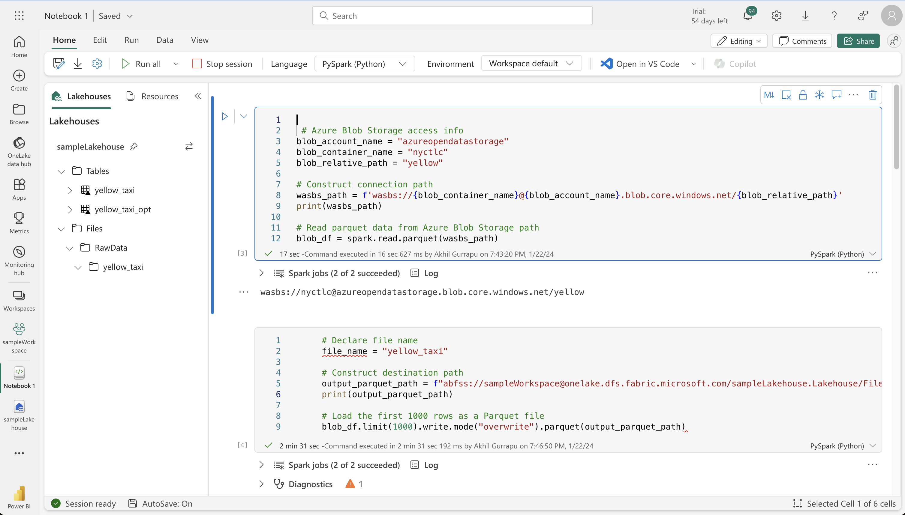
Loading External Data
 # Azure Blob Storage access info
blob_account_name = "azureopendatastorage"
blob_container_name = "nyctlc"
blob_relative_path = "yellow"

# Construct connection path
wasbs_path = f'wasbs://{blob_container_name}@{blob_account_name}.blob.core.windows.net/{blob_relative_path}'
print(wasbs_path)

# Read parquet data from Azure Blob Storage path
blob_df = spark.read.parquet(wasbs_path)
StatementMeta(, 57c76e74-4270-48f9-bbfa-69e43c451477, 5, Finished, Available)
wasbs://nyctlc@azureopendatastorage.blob.core.windows.net/yellow
     # Declare file name
     file_name = "yellow_taxi"

     # Construct destination path
     output_parquet_path = f"abfss://sampleWorkspace@onelake.dfs.fabric.microsoft.com/sampleLakehouse.Lakehouse/Files/RawData/{file_name}"
     print(output_parquet_path)

     # Load the first 1000 rows as a Parquet file
     blob_df.limit(1000).write.mode("overwrite").parquet(output_parquet_path)
StatementMeta(, 57c76e74-4270-48f9-bbfa-69e43c451477, 6, Finished, Available)
abfss://sampleWorkspace@onelake.dfs.fabric.microsoft.com/sampleLakehouse.Lakehouse/Files/RawData/yellow_taxi
Transforming and loading data to a Delta table
from pyspark.sql.functions import col, to_timestamp, current_timestamp, year, month

raw_df = spark.read.parquet(output_parquet_path)

filtered_df = raw_df.withColumn("dataload_datetime", current_timestamp())

filtered_df = raw_df.filter(raw_df["storeAndFwdFlag"].isNotNull())

table_name = "yellow_taxi"

filtered_df.write.format("delta").mode("append").saveAsTable(table_name)

display(filtered_df.limit(5))
StatementMeta(, 57c76e74-4270-48f9-bbfa-69e43c451477, 8, Finished, Available)
| vendorID | tpepPickupDateTime | tpepDropoffDateTime | passengerCount | tripDistance | puLocationId | doLocationId | startLon | startLat | endLon | endLat | rateCodeId | storeAndFwdFlag | paymentType | fareAmount | extra | mtaTax | improvementSurcharge | tipAmount | tollsAmount | totalAmount | puYear | puMonth |
|----------|-----------------------|-----------------------|----------------|--------------|--------------|--------------|------------|-----------|-----------|----------|------------|-----------------|-------------|------------|-------|--------|----------------------|-----------|-------------|-------------|--------|---------|
| CMT | 2012-02-29 23:57:57 | 2012-03-01 00:07:31 | 1 | 2.5 | NULL | NULL | -73.949531 | 40.78098 | -73.975767| 40.755122| 1 | N | CRD | 8.5 | 0.5 | 0.5 | NULL | 1.0 | 0.0 | 10.5 | 2012 | 3 |
| CMT | 2012-02-29 23:55:46 | 2012-03-01 00:05:02 | 1 | 1.8 | NULL | NULL | -74.006604| 40.739769 | -73.994188| 40.758891| 1 | N | CRD | 7.7 | 0.5 | 0.5 | NULL | 1.0 | 0.0 | 9.7 | 2012 | 3 |
| CMT | 2012-03-01 17:35:10 | 2012-03-01 17:55:46 | 1 | 1.5 | NULL | NULL | -73.968988| 40.757481 | -73.986903| 40.750641| 1 | N | CRD | 11.3 | 1.0 | 0.5 | NULL | 1.0 | 0.0 | 13.8 | 2012 | 3 |
| CMT | 2012-03-03 13:52:50 | 2012-03-03 14:02:33 | 2 | 2.1 | NULL | NULL | -73.965915| 40.805511 | -73.972544| 40.781006| 1 | N | CRD | 8.1 | 0.0 | 0.5 | NULL | 1.0 | 0.0 | 9.6 | 2012 | 3 |
| CMT | 2012-03-02 07:33:59 | 2012-03-02 07:40:23 | 1 | 1.3 | NULL | NULL | -73.981007| 40.755079 | -73.968284| 40.768198| 1 | N | CRD | 5.7 | 0.0 | 0.5 | NULL | 1.0 | 0.0 | 7.2 | 2012 | 3 |
Optimizing Delta table writes
 from pyspark.sql.functions import col, to_timestamp, current_timestamp, year, month

 # Read the parquet data from the specified path
 raw_df = spark.read.parquet(output_parquet_path)

 # Add dataload_datetime column with current timestamp
 opt_df = raw_df.withColumn("dataload_datetime", current_timestamp())

 # Filter columns to exclude any NULL values in storeAndFwdFlag
 opt_df = opt_df.filter(opt_df["storeAndFwdFlag"].isNotNull())

 # Enable V-Order
 spark.conf.set("spark.sql.parquet.vorder.enabled", "true")

 # Enable automatic Delta optimized write
 spark.conf.set("spark.microsoft.delta.optimizeWrite.enabled", "true")

 # Load the filtered data into a Delta table
 table_name = "yellow_taxi_opt"  # New table name
 opt_df.write.format("delta").mode("append").saveAsTable(table_name)

 # Display results
 display(opt_df.limit(5))
StatementMeta(, 57c76e74-4270-48f9-bbfa-69e43c451477, 9, Finished, Available)
| vendorID | tpepPickupDateTime | tpepDropoffDateTime | passengerCount | tripDistance | puLocationId | doLocationId | startLon | startLat | endLon | endLat | rateCodeId | storeAndFwdFlag | paymentType | fareAmount | extra | mtaTax | improvementSurcharge | tipAmount | tollsAmount | totalAmount | puYear | puMonth |
|----------|-----------------------|-----------------------|----------------|--------------|--------------|--------------|------------|-----------|-----------|----------|------------|-----------------|-------------|------------|-------|--------|----------------------|-----------|-------------|-------------|--------|---------|
| CMT | 2012-02-29 23:57:57 | 2012-03-01 00:07:31 | 1 | 2.5 | NULL | NULL | -73.949531 | 40.78098 | -73.975767| 40.755122| 1 | N | CRD | 8.5 | 0.5 | 0.5 | NULL | 1.0 | 0.0 | 10.5 | 2012 | 3 |
| CMT | 2012-02-29 23:55:46 | 2012-03-01 00:05:02 | 1 | 1.8 | NULL | NULL | -74.006604| 40.739769 | -73.994188| 40.758891| 1 | N | CRD | 7.7 | 0.5 | 0.5 | NULL | 1.0 | 0.0 | 9.7 | 2012 | 3 |
| CMT | 2012-03-01 17:35:10 | 2012-03-01 17:55:46 | 1 | 1.5 | NULL | NULL | -73.968988| 40.757481 | -73.986903| 40.750641| 1 | N | CRD | 11.3 | 1.0 | 0.5 | NULL | 1.0 | 0.0 | 13.8 | 2012 | 3 |
| CMT | 2012-03-03 13:52:50 | 2012-03-03 14:02:33 | 2 | 2.1 | NULL | NULL | -73.965915| 40.805511 | -73.972544| 40.781006| 1 | N | CRD | 8.1 | 0.0 | 0.5 | NULL | 1.0 | 0.0 | 9.6 | 2012 | 3 |
| CMT | 2012-03-02 07:33:59 | 2012-03-02 07:40:23 | 1 | 1.3 | NULL | NULL | -73.981007| 40.755079 | -73.968284| 40.768198| 1 | N | CRD | 5.7 | 0.0 | 0.5 | NULL | 1.0 | 0.0 | 7.2 | 2012 | 3 |
Analyzing Delta table data with SQL queries
table_name = "yellow_taxi"

df = spark.read.format("delta").table(table_name)


df.createOrReplaceTempView("tempView")


query = "SELECT * FROM tempView"

newDF = spark.sql(query)

display(newDF.limit(3))
StatementMeta(, 57c76e74-4270-48f9-bbfa-69e43c451477, 13, Finished, Available)
| vendorID | tpepPickupDateTime | tpepDropoffDateTime | passengerCount | tripDistance | puLocationId | doLocationId | startLon | startLat | endLon | endLat | rateCodeId | storeAndFwdFlag | paymentType | fareAmount | extra | mtaTax | improvementSurcharge | tipAmount | tollsAmount | totalAmount | puYear | puMonth |
|----------|-----------------------|-----------------------|----------------|--------------|--------------|--------------|------------|-----------|-----------|----------|------------|-----------------|-------------|------------|-------|--------|----------------------|-----------|-------------|-------------|--------|---------|
| CMT | 2012-02-29 23:57:57 | 2012-03-01 00:07:31 | 1 | 2.5 | NULL | NULL | -73.949531 | 40.78098 | -73.975767| 40.755122| 1 | N | CRD | 8.5 | 0.5 | 0.5 | NULL | 1.0 | 0.0 | 10.5 | 2012 | 3 |
| CMT | 2012-02-29 23:55:46 | 2012-03-01 00:05:02 | 1 | 1.8 | NULL | NULL | -74.006604| 40.739769 | -73.994188| 40.758891| 1 | N | CRD | 7.7 | 0.5 | 0.5 | NULL | 1.0 | 0.0 | 9.7 | 2012 | 3 |
| CMT | 2012-03-01 17:35:10 | 2012-03-01 17:55:46 | 1 | 1.5 | NULL | NULL | -73.968988| 40.757481 | -73.986903| 40.750641| 1 | N | CRD | 11.3 | 1.0 | 0.5 | NULL | 1.0 | 0.0 | 13.8 | 2012 | 3 |