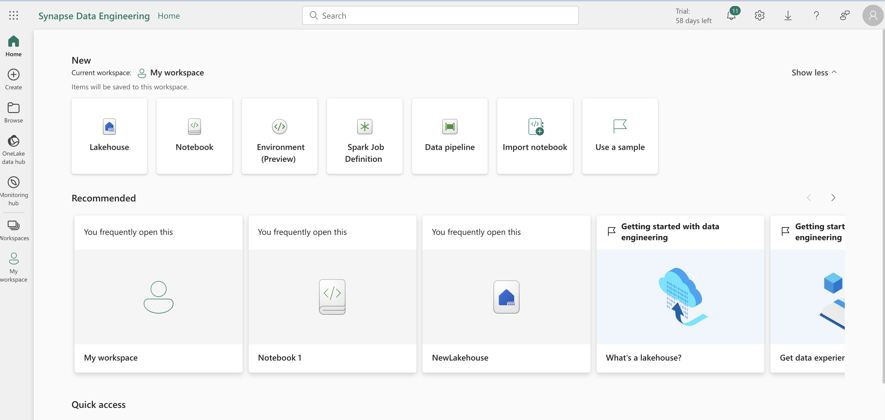
Exploring Sales Data with Apache Spark in Synapse Data Engineering
In this tutorial, we navigate the process of creating a lakehouse in Synapse Data Engineering, a critical component for data analysis and management. The journey begins by downloading a dataset (orders.zip) containing sales data from 2019 to 2021 in CSV format. After uploading these files to the newly created lakehouse, we dive into data exploration using Apache Spark within Synapse.

Exploring Sales Data with Apache Spark in Synapse Data Engineering
-
In this tutorial, we navigate the process of creating a lakehouse in Synapse Data Engineering, a critical component for data analysis and management. The journey begins by downloading a dataset (orders.zip) containing sales data from 2019 to 2021 in CSV format. After uploading these files to the newly created lakehouse, we dive into data exploration using Apache Spark within Synapse.
-
Download and extract the data files for this exercise from https://github.com/MicrosoftLearning/dp-data/raw/main/orders.zip.
Data Loading and Transformation
- Initially, the data is loaded without headers, requiring a modification to include headers for clarity. Then, we define a schema to correctly interpret the data types in our CSV files. This schema includes fields like SalesOrderNumber, CustomerName, Item, etc. The dataframe is further enhanced to read all CSV files using a wildcard (*), ensuring the inclusion of data from 2019 to 2021.
# Reading the files uploaded in the lakehouse using pyspark
# loading the data into the dataframe

df = spark.read.format("csv").option("header","false").load("Files/orders/2019.csv")

display(df)
StatementMeta(, 1b68eedb-c823-4c31-bc2c-bf23ad10ea64, 5, Finished, Available)
SynapseWidget(Synapse.DataFrame, 2a78e328-1f2e-4edb-a092-33c7027bdbbf)
Defining a Schema and applying it when loading the data
from pyspark.sql.types import *

orderSchema = StructType([
    StructField("SalesOrderNumber", StringType()),
    StructField("SalesOrderLineNumber", IntegerType()),
    StructField("OrderDate", DateType()),
    StructField("CustomerName", StringType()),
    StructField("Email", StringType()),
    StructField("Item", StringType()),
    StructField("Quantity", IntegerType()),
    StructField("UnitPrice", FloatType()),
    StructField("Tax", FloatType())
    ])

df = spark.read.format("csv").schema(orderSchema).load("Files/orders/2019.csv")
display(df)
StatementMeta(, 1b68eedb-c823-4c31-bc2c-bf23ad10ea64, 32, Finished, Available)
SynapseWidget(Synapse.DataFrame, 21b64a97-d84a-407f-bbb6-219c32c646bb)
df.count()StatementMeta(, 1b68eedb-c823-4c31-bc2c-bf23ad10ea64, 33, Finished, Available)
1201
A ‘*’ wildcard to read the sales order data from all of the files in the orders folder: ***
from pyspark.sql.types import *

orderSchema = StructType([
   StructField("SalesOrderNumber", StringType()),
   StructField("SalesOrderLineNumber", IntegerType()),
   StructField("OrderDate", DateType()),
   StructField("CustomerName", StringType()),
   StructField("Email", StringType()),
   StructField("Item", StringType()),
   StructField("Quantity", IntegerType()),
   StructField("UnitPrice", FloatType()),
   StructField("Tax", FloatType())
   ])

df = spark.read.format("csv").schema(orderSchema).load("Files/orders/*.csv")
display(df)
StatementMeta(, 1b68eedb-c823-4c31-bc2c-bf23ad10ea64, 34, Finished, Available)
SynapseWidget(Synapse.DataFrame, d0a6bdba-b070-40de-93c0-bea3c3ec789e)
df.count()StatementMeta(, 1b68eedb-c823-4c31-bc2c-bf23ad10ea64, 35, Finished, Available)
32718
Dataframe Operations: Filtering, Aggregating, and Grouping
- We employ dataframe operations to manipulate and understand the data better. These include filtering to view specific customer data, aggregating sales data, and grouping by product or year. For example, we group sales data by product item and sum the quantities to understand product popularity.
customers = df['CustomerName', 'Email']
print(customers.count())
print(customers.distinct().count())
display(customers.distinct())
StatementMeta(, 1b68eedb-c823-4c31-bc2c-bf23ad10ea64, 36, Finished, Available)
32718
12427
SynapseWidget(Synapse.DataFrame, 7633bd80-3832-48bc-9c77-c5e09db9e4bd)
customers = df.select("CustomerName", "Email").where(df['Item']=='Road-250 Red, 52')
print(customers.count())
print(customers.distinct().count())
display(customers.distinct())
StatementMeta(, 1b68eedb-c823-4c31-bc2c-bf23ad10ea64, 37, Finished, Available)
133
133
SynapseWidget(Synapse.DataFrame, 49faf4a0-fcce-47be-8f99-3b637df455b8)
Aggregate and group data in a dataframe
productSales = df.select("Item", "Quantity").groupBy("Item").sum()
display(productSales)
StatementMeta(, 1b68eedb-c823-4c31-bc2c-bf23ad10ea64, 38, Finished, Available)
SynapseWidget(Synapse.DataFrame, edc501fc-90ae-41ec-8ff9-be43630c604c)
from pyspark.sql.functions import *

yearlySales = df.select(year(col("OrderDate")).alias("Year")).groupBy("Year").count().orderBy("Year")
display(yearlySales)
StatementMeta(, 1b68eedb-c823-4c31-bc2c-bf23ad10ea64, 39, Finished, Available)
SynapseWidget(Synapse.DataFrame, f2ca4605-1597-4e5e-9716-bc9795b39471)
Transforming and Storing Data
- A crucial step in data engineering is transforming data for downstream processing. We add new columns like Year and Month, split CustomerName into FirstName and LastName, and reorder the columns. The transformed data is then stored in a Parquet format, an efficient format for large-scale data analytics.
from pyspark.sql.functions import *

## Create Year and Month columns
transformed_df = df.withColumn("Year", year(col("OrderDate"))).withColumn("Month", month(col("OrderDate")))

# Create the new FirstName and LastName fields
transformed_df = transformed_df.withColumn("FirstName", split(col("CustomerName"), " ").getItem(0)).withColumn("LastName", split(col("CustomerName"), " ").getItem(1))

# Filter and reorder columns
transformed_df = transformed_df["SalesOrderNumber", "SalesOrderLineNumber", "OrderDate", "Year", "Month", "FirstName", "LastName", "Email", "Item", "Quantity", "UnitPrice", "Tax"]

# Display the first five orders
display(transformed_df.limit(5))
StatementMeta(, 1b68eedb-c823-4c31-bc2c-bf23ad10ea64, 40, Finished, Available)
SynapseWidget(Synapse.DataFrame, 89a777e8-153a-4920-a754-1a16da521317)
transformed_df.write.mode("overwrite").parquet('Files/transformed_data/orders')
print ("Transformed data saved!")
StatementMeta(, 1b68eedb-c823-4c31-bc2c-bf23ad10ea64, 41, Finished, Available)
Transformed data saved!
orders_df = spark.read.format("parquet").load("Files/transformed_data/orders")
display(orders_df)
StatementMeta(, 1b68eedb-c823-4c31-bc2c-bf23ad10ea64, 45, Finished, Available)
SynapseWidget(Synapse.DataFrame, 448689a4-4c53-4c9b-93a8-0e9eeec06f1d)
orders_df.write.partitionBy("Year","Month").mode("overwrite").parquet("Files/partitioned_data")
print ("Transformed data saved!")
StatementMeta(, 1b68eedb-c823-4c31-bc2c-bf23ad10ea64, 46, Finished, Available)
Transformed data saved!
Partitioning and Loading Data
- To enhance performance, the data is saved in a partitioned format by Year and Month. We then load specific subsets of this data, like sales for the year 2021, demonstrating the efficiency of partitioned data.
orders_2019_df = spark.read.format("parquet").load("Files/partitioned_data/Year=2019/Month=*")
display(orders_2019_df)
StatementMeta(, 1b68eedb-c823-4c31-bc2c-bf23ad10ea64, 42, Finished, Available)
SynapseWidget(Synapse.DataFrame, 638602ca-580e-434b-8bdc-63516aad15db)
Working with Tables and SQL in Spark
For users more comfortable with SQL, Spark offers the flexibility of defining relational tables and querying them using SQL syntax. We create a salesorders table, save it in delta format, and execute SQL queries to analyze data like calculating gross revenue per year.
# Create a new table
df.write.format("delta").saveAsTable("sales_orders")

# Get the table description
spark.sql("DESCRIBE EXTENDED sales_orders").show(truncate=False)
StatementMeta(, 1b68eedb-c823-4c31-bc2c-bf23ad10ea64, 48, Finished, Available)
+----------------------------+--------------------------------------------------------------------------------------------------------------------------------------+-------+
|col_name |data_type |comment|
+----------------------------+--------------------------------------------------------------------------------------------------------------------------------------+-------+
|SalesOrderNumber |string |null |
|SalesOrderLineNumber |int |null |
|OrderDate |date |null |
|CustomerName |string |null |
|Email |string |null |
|Item |string |null |
|Quantity |int |null |
|UnitPrice |float |null |
|Tax |float |null |
| | | |
|# Detailed Table Information| | |
|Name |spark_catalog.newlakehouse.sales_orders | |
|Type |MANAGED | |
|Location |abfss://11baa5af-8529-42b1-a519-0b07ec9aaab4@onelake.dfs.fabric.microsoft.com/8fc37f8f-7236-41ee-923b-6797f693e8fd/Tables/sales_orders| |
|Provider |delta | |
|Owner |trusted-service-user | |
|Table Properties |[delta.minReaderVersion=1,delta.minWriterVersion=2] | |
+----------------------------+--------------------------------------------------------------------------------------------------------------------------------------+-------+
df = spark.sql("SELECT * FROM NewLakehouse.sales_orders LIMIT 100")
display(df)
StatementMeta(, 1b68eedb-c823-4c31-bc2c-bf23ad10ea64, 49, Finished, Available)
SynapseWidget(Synapse.DataFrame, d95df6a5-44fe-426e-8fee-e419445f7be4)
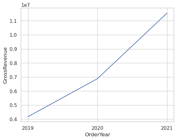
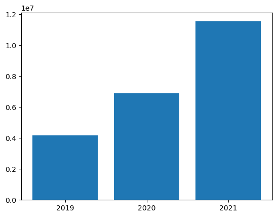
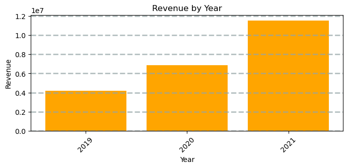
Visualizing Data with Spark and Python Libraries
Finally, we delve into data visualization using Spark’s built-in chart view and Python libraries like matplotlib and seaborn. These tools allow us to create compelling visual representations of our data, such as bar and line charts, enhancing our understanding and presentation of the data insights.
sqlQuery = "SELECT CAST(YEAR(OrderDate) AS CHAR(4)) AS OrderYear, \
                SUM((UnitPrice * Quantity) + Tax) AS GrossRevenue \
            FROM sales_orders \
            GROUP BY CAST(YEAR(OrderDate) AS CHAR(4)) \
            ORDER BY OrderYear"
df_spark = spark.sql(sqlQuery)
df_spark.show()
StatementMeta(, 1b68eedb-c823-4c31-bc2c-bf23ad10ea64, 50, Finished, Available)
+---------+--------------------+
|OrderYear| GrossRevenue|
+---------+--------------------+
| 2019| 4172169.969970703|
| 2020| 6882259.268127441|
| 2021|1.1547835291696548E7|
+---------+--------------------+
from matplotlib import pyplot as plt

# matplotlib requires a Pandas dataframe, not a Spark one
df_sales = df_spark.toPandas()

# Create a bar plot of revenue by year
plt.bar(x=df_sales['OrderYear'], height=df_sales['GrossRevenue'])

# Display the plot
plt.show()
StatementMeta(, 1b68eedb-c823-4c31-bc2c-bf23ad10ea64, 51, Finished, Available)
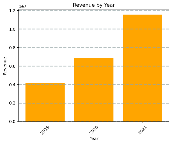
from matplotlib import pyplot as plt

# Clear the plot area
plt.clf()

# Create a bar plot of revenue by year
plt.bar(x=df_sales['OrderYear'], height=df_sales['GrossRevenue'], color='orange')

# Customize the chart
plt.title('Revenue by Year')
plt.xlabel('Year')
plt.ylabel('Revenue')
plt.grid(color='#95a5a6', linestyle='--', linewidth=2, axis='y', alpha=0.7)
plt.xticks(rotation=45)

# Show the figure
plt.show()
StatementMeta(, 1b68eedb-c823-4c31-bc2c-bf23ad10ea64, 52, Finished, Available)
from matplotlib import pyplot as plt

# Clear the plot area
plt.clf()

# Create a Figure
fig = plt.figure(figsize=(8,3))

# Create a bar plot of revenue by year
plt.bar(x=df_sales['OrderYear'], height=df_sales['GrossRevenue'], color='orange')

# Customize the chart
plt.title('Revenue by Year')
plt.xlabel('Year')
plt.ylabel('Revenue')
plt.grid(color='#95a5a6', linestyle='--', linewidth=2, axis='y', alpha=0.7)
plt.xticks(rotation=45)

# Show the figure
plt.show()
StatementMeta(, 1b68eedb-c823-4c31-bc2c-bf23ad10ea64, 53, Finished, Available)
<Figure size 640x480 with 0 Axes>
from matplotlib import pyplot as plt
# Clear the plot area
plt.clf()
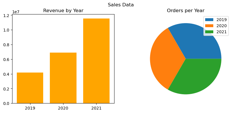
# Create a figure for 2 subplots (1 row, 2 columns)
fig, ax = plt.subplots(1, 2, figsize = (10,4))
# Create a bar plot of revenue by year on the first axis
ax[0].bar(x=df_sales['OrderYear'], height=df_sales['GrossRevenue'], color='orange')
ax[0].set_title('Revenue by Year')
# Create a pie chart of yearly order counts on the second axis
yearly_counts = df_sales['OrderYear'].value_counts()
ax[1].pie(yearly_counts)
ax[1].set_title('Orders per Year')
ax[1].legend(yearly_counts.keys().tolist())
# Add a title to the Figure
fig.suptitle('Sales Data')
# Show the figure
plt.show()StatementMeta(, 1b68eedb-c823-4c31-bc2c-bf23ad10ea64, 54, Finished, Available)
<Figure size 640x480 with 0 Axes>
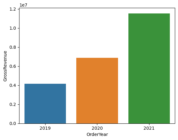
Using Seaborn Library
import seaborn as sns

# Clear the plot area
plt.clf()

# Create a bar chart
ax = sns.barplot(x="OrderYear", y="GrossRevenue", data=df_sales)
plt.show()
StatementMeta(, 1b68eedb-c823-4c31-bc2c-bf23ad10ea64, 55, Finished, Available)
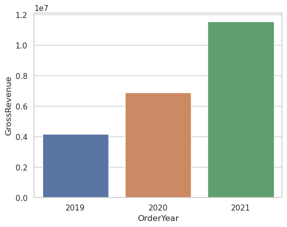
import seaborn as sns

# Clear the plot area
plt.clf()

# Set the visual theme for seaborn
sns.set_theme(style="whitegrid")

# Create a bar chart
ax = sns.barplot(x="OrderYear", y="GrossRevenue", data=df_sales)
plt.show()
StatementMeta(, 1b68eedb-c823-4c31-bc2c-bf23ad10ea64, 56, Finished, Available)
import seaborn as sns

# Clear the plot area
plt.clf()

# Create a line chart
ax = sns.lineplot(x="OrderYear", y="GrossRevenue", data=df_sales)
plt.show()
StatementMeta(, 1b68eedb-c823-4c31-bc2c-bf23ad10ea64, 57, Finished, Available)