Apache Spark in Microsoft Fabric

Spark

Apache Spark has emerged as a leading open-source framework for large-scale data processing, especially in the realm of “big data”. Its adaptability across various platforms, including Azure HDInsight, Azure Databricks, Azure Synapse Analytics, and Microsoft Fabric, has contributed to its popularity.

Focusing on Microsoft Fabric, this powerful tool integrates seamlessly with Spark to enhance data ingestion, processing, and analysis in a lakehouse environment. The core techniques and code used in Spark are universally applicable across its different implementations. However, the unique advantage of Microsoft Fabric lies in its integration of Spark with other data services.

Explore more about Spark architecture and more in this blog.

Key Features of Apache Spark in Microsoft Fabric

1. Language Support: Spark supports various languages including Java, Scala, Spark R, Spark SQL, and PySpark. The latter two are most commonly used for data engineering and analytics tasks.

2. Spark Settings in Microsoft Fabric: Each workspace in Microsoft Fabric is assigned a Spark cluster, with settings manageable under the Data Engineering/Science section. Key settings include:

   • Node Family: Generally, memory-optimized nodes are preferred for optimal performance.
   • Runtime Version: Determines the Spark version and its subcomponents.
   • Spark Properties: Customizable settings based on Apache Spark documentation. Default settings usually suffice in most cases.

3. Libraries: Spark benefits from a rich ecosystem of open-source libraries, especially in Python, ensuring support for a wide array of tasks. Microsoft Fabric’s Spark clusters come pre-loaded with common libraries, and additional libraries can be managed on the library management page.

Exploring and Running Spark Code in Microsoft Fabric: A Quick Guide

Microsoft Fabric offers two primary ways to work with Spark code: through notebooks and Spark job definitions.

1. Notebooks for Interactive Analysis:

   • Ideal for interactive data exploration and analysis.
   • Notebooks in Microsoft Fabric are versatile, allowing you to combine text, images, and code in multiple languages. This creates a dynamic and collaborative environment.
   • You can interactively run code within these notebooks and see immediate results. Each notebook is made up of cells that can either contain markdown-formatted content or executable code.

2. Spark Job Definitions for Automated Processes:

   • Best suited for automating data ingestion and transformation tasks.
   • Define a Spark job in your workspace, specifying the script to be run either on-demand or on a schedule.
   • Additional Configuration: Options include adding reference files (like Python code files) and specifying a particular lakehouse for data processing.

In summary, Microsoft Fabric provides flexible options for both interactive data analysis and automated data processing with Spark, catering to different needs and workflows.

Working with data in Apache Spark often involves using dataframes, an essential part of the Spark SQL library. Unlike the low-level resilient distributed dataset (RDD), dataframes offer a more intuitive and structured approach to data manipulation, especially for those familiar with the popular Pandas library in Python.

Loading Data into a Dataframe

• Consider a scenario where you have a CSV file (products.csv) with product data. In Spark, you can load this file into a dataframe with just a few lines of PySpark code:

%%pyspark
df = spark.read.load('Files/data/products.csv',
    format='csv',
    header=True
)
display(df.limit(10))

StatementMeta(, fbe6de24-8e0c-4c1a-9b70-0926d42e7ce7, 4, Finished, Available)



SynapseWidget(Synapse.DataFrame, f125a8e9-69c3-4c47-9979-bf3da50cdfd5)

Loading Data into a Dataframe

• Consider a scenario where you have a CSV file (products.csv) with product data. In Spark, you can load this file into a dataframe with just a few lines of PySpark code:

from pyspark.sql.types import *
from pyspark.sql.functions import *

productSchema = StructType([
    StructField("ProductID", IntegerType()),
    StructField("ProductName", StringType()),
    StructField("Category", StringType()),
    StructField("ListPrice", FloatType())
    ])

df = spark.read.load('Files/data/products-data.csv',
    format='csv',
    schema=productSchema,
    header=False)
display(df.limit(10))

StatementMeta(, 1a7b1439-f087-4da5-9cf4-c776ec4f2ad3, 7, Finished, Available)



SynapseWidget(Synapse.DataFrame, 3d6a2160-5bc9-43d5-85c3-353d091b0063)

Data Manipulation: Filtering and Grouping

• Spark dataframes allow for various data manipulations like filtering, sorting, and grouping. For instance, you can select specific columns or filter data based on conditions:

pricelist_df = df.select("ProductID", "ListPrice")
bikes_df = df.select("ProductName", "Category", "ListPrice").where((df["Category"]=="Mountain Bikes") | (df["Category"]=="Road Bikes"))
display(bikes_df)

StatementMeta(, 1a7b1439-f087-4da5-9cf4-c776ec4f2ad3, 9, Finished, Available)



SynapseWidget(Synapse.DataFrame, 06901126-059b-4307-a513-4b0e3f42d07d)

• To group and aggregate data, you can use the groupBy method and aggregate functions. For example, the following PySpark code counts the number of products for each category:

counts_df = df.select("ProductID", "Category").groupBy("Category").count()
display(counts_df)

StatementMeta(, 1a7b1439-f087-4da5-9cf4-c776ec4f2ad3, 10, Finished, Available)



SynapseWidget(Synapse.DataFrame, 807d83e5-6264-455a-98e5-d13c6a757d5c)

Saving Dataframes

• After data transformation, you might need to save your results. Spark allows you to save dataframes in various formats, including Parquet, a preferred format for analytics due to its efficiency:

bikes_df.write.mode("overwrite").parquet('Files/product_data/bikes.parquet')

StatementMeta(, 1a7b1439-f087-4da5-9cf4-c776ec4f2ad3, 11, Finished, Available)

Partitioning for Performance

• Partitioning data when saving it can significantly improve performance. This approach organizes data into folders based on specific column values, making future data operations more efficient:

bikes_df.write.partitionBy("Category").mode("overwrite").parquet("Files/bike_data")

StatementMeta(, 1a7b1439-f087-4da5-9cf4-c776ec4f2ad3, 12, Finished, Available)

Loading Partitioned Data

• When reading partitioned data, Spark allows you to specify which partitions to load, enhancing the efficiency of data reads:

road_bikes_df = spark.read.parquet('Files/bike_data/Category=Road Bikes')

Spark SQL: Simplifying Data Analysis in Spark

• Spark SQL is a powerful tool within Apache Spark, designed to make data analysis simpler and more accessible. It integrates seamlessly with Spark’s Dataframe API, allowing data analysts and developers to query and manipulate data using SQL expressions.

Creating Views and Tables in Spark Catalog

• The Spark catalog serves as a repository for relational data objects like views and tables. By creating a temporary view from a dataframe, users can easily query the data. However, these views are temporary and are deleted when the session ends.

df.createOrReplaceTempView("products_view")

StatementMeta(, fbe6de24-8e0c-4c1a-9b70-0926d42e7ce7, 5, Finished, Available)

• For more permanent solutions, Spark allows the creation of tables, which are stored in the Spark catalog. These tables can be created either by defining an empty table or by saving a dataframe as a table, as shown in the command df.write.format(“delta”).saveAsTable(“products”). It’s important to note that deleting a managed table will also remove its underlying data.

df.write.format("delta").saveAsTable("products")

StatementMeta(, fbe6de24-8e0c-4c1a-9b70-0926d42e7ce7, 6, Finished, Available)

Querying Data with Spark SQL API

• The Spark SQL API allows querying data in any supported language. For instance, querying data from a table into a dataframe can be done using:

bikes_df = spark.sql("SELECT ProductID, ProductName, ListPrice FROM products WHERE Category IN ('Mountain Bikes', 'Road Bikes')")
display(bikes_df)

StatementMeta(, fbe6de24-8e0c-4c1a-9b70-0926d42e7ce7, 7, Finished, Available)



SynapseWidget(Synapse.DataFrame, d286dea1-945e-4c91-974e-172790a6e3f8)

Using SQL in Notebooks

Within notebooks, the %%sql magic command can be used to directly run SQL code. This is particularly useful for querying and displaying data from the catalog in a straightforward and readable format.

%%sql

SELECT Category, COUNT(ProductID) AS ProductCount
FROM products
GROUP BY Category
ORDER BY Category

StatementMeta(, fbe6de24-8e0c-4c1a-9b70-0926d42e7ce7, 14, Finished, Available)





<Spark SQL result set with 2 rows and 2 fields>

from matplotlib import pyplot as plt
import pandas as pd
import numpy as np

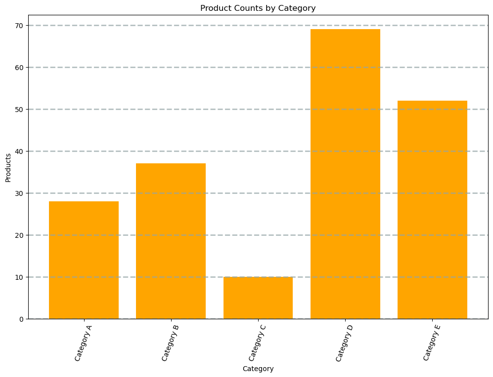
# Generate random data for demonstration
categories = ['Category A', 'Category B', 'Category C', 'Category D', 'Category E']
product_counts = np.random.randint(1, 100, size=len(categories))

# Create a DataFrame from the generated data
data = pd.DataFrame({'Category': categories, 'ProductCount': product_counts})

# Clear the plot area
plt.clf()

# Create a Figure
fig = plt.figure(figsize=(12, 8))

# Create a bar plot of product counts by category
plt.bar(x=data['Category'], height=data['ProductCount'], color='orange')

# Customize the chart
plt.title('Product Counts by Category')
plt.xlabel('Category')
plt.ylabel('Products')
plt.grid(color='#95a5a6', linestyle='--', linewidth=2, axis='y', alpha=0.7)
plt.xticks(rotation=70)

# Show the plot area
plt.show()

StatementMeta(, fbe6de24-8e0c-4c1a-9b70-0926d42e7ce7, 19, Finished, Available)



<Figure size 640x480 with 0 Axes>